Working with SBML Ids
Usually basico uses the COPASI display names, to work with model elements. That way a consistent naming scheme between the COPASI graphical user interface, and the scripts can be easily maintained. However, for someone inspecting an SBML model, it might be convenient to also look at the SBML ids and identify elements that way. For this reason the data frames returned for compartments, events, parameters, species and reactions now also contain a column sbml_id.
Lets start as usual with the common imports:
[1]:
import sys
if '../..' not in sys.path:
    sys.path.append('../..')
from basico import *
import numpy as np
import matplotlib.pyplot as plt
%matplotlib inline
Next lets load a model from the BioModels Database, and look at the elments:
[2]:
load_biomodel(64);
Now we have not just the element name availabe, but also their respective sbml_id:
[3]:
get_species()[['sbml_id', 'initial_concentration']]
[3]:
| sbml_id | initial_concentration | |
|---|---|---|
| name | ||
| High energy phosphates | P | 6.310000 |
| Glucose 6 Phosphate | G6P | 2.450000 |
| Triose-phosphate | TRIO | 0.960000 |
| NAD | NAD | 1.200000 |
| Acetaldehyde | ACE | 0.170000 |
| 2-phosphoglycerate | P2G | 0.120000 |
| 1,3-bisphosphoglycerate | BPG | 0.000000 |
| Glucose in Cytosol | GLCi | 0.087000 |
| Fructose 6 Phosphate | F6P | 0.620000 |
| Phosphoenolpyruvate | PEP | 0.070000 |
| Pyruvate | PYR | 1.850000 |
| Fructose-1,6 bisphosphate | F16P | 5.510000 |
| 3-phosphoglycerate | P3G | 0.900000 |
| NADH | NADH | 0.390000 |
| ATP concentration | ATP | 2.509190 |
| ADP concentration | ADP | 1.291619 |
| AMP concentration | AMP | 0.299190 |
| Extracellular Glucose | GLCo | 50.000000 |
| Glycogen | Glyc | 0.000000 |
| Trehalose | Trh | 0.000000 |
| CO2 | CO2 | 1.000000 |
| Succinate | SUCC | 0.000000 |
| Ethanol | ETOH | 50.000000 |
| Glycerol | GLY | 0.150000 |
| sum of AXP conc | SUM_P | 4.100000 |
| F2,6P | F26BP | 0.020000 |
similarly we can get the elements by SBML id as well:
[4]:
get_species(sbml_id='ATP')
[4]:
| compartment | type | unit | initial_concentration | initial_particle_number | initial_expression | expression | concentration | particle_number | rate | particle_number_rate | key | sbml_id | |
|---|---|---|---|---|---|---|---|---|---|---|---|---|---|
| name | |||||||||||||
| ATP concentration | cytosol | assignment | mmol/l | 2.50919 | 1.511070e+21 | ( [High energy phosphates] - [ADP concentratio... | NaN | NaN | NaN | NaN | Metabolite_21 | ATP |
Whereas in COPASI each element has a concentration and a particle number, in SBML usually elements deal only with concentrations and amounts. To make it easy to access them, it is convenient to add the expressions for the amount to the model, so that they can be accessed at any point in time. For that a utility function exists. If use_sbml_ids is specified, the sbml id of the species will be used in the name (i.e: amount(sbml_id)), otherwise it will be named amount(display name). In
case ignore_fixed is specified, no expressions for fixed species will be created, and similarly assignment expressions can be ignored:
[5]:
add_amount_expressions(use_sbml_ids=True, ignore_fixed=True)
lets look at the expressions created, we see it is just the concentration multiplied with the compartment size the species is in:
[6]:
get_parameters(name='amount(')[['initial_value', 'expression']]
[6]:
| initial_value | expression | |
|---|---|---|
| name | ||
| amount(GLCi) | 0.087000 | [Glucose in Cytosol] * Compartments[cytosol].V... |
| amount(G6P) | 2.450000 | [Glucose 6 Phosphate] * Compartments[cytosol].... |
| amount(F6P) | 0.620000 | [Fructose 6 Phosphate] * Compartments[cytosol]... |
| amount(F16P) | 5.510000 | [Fructose-1,6 bisphosphate] * Compartments[cyt... |
| amount(TRIO) | 0.960000 | [Triose-phosphate] * Compartments[cytosol].Volume |
| amount(BPG) | 0.000000 | [1,3-bisphosphoglycerate] * Compartments[cytos... |
| amount(P3G) | 0.900000 | [3-phosphoglycerate] * Compartments[cytosol].V... |
| amount(P2G) | 0.120000 | [2-phosphoglycerate] * Compartments[cytosol].V... |
| amount(PEP) | 0.070000 | [Phosphoenolpyruvate] * Compartments[cytosol].... |
| amount(PYR) | 1.850000 | [Pyruvate] * Compartments[cytosol].Volume |
| amount(ACE) | 0.170000 | [Acetaldehyde] * Compartments[cytosol].Volume |
| amount(P) | 6.310000 | [High energy phosphates] * Compartments[cytoso... |
| amount(NAD) | 1.200000 | [NAD] * Compartments[cytosol].Volume |
| amount(NADH) | 0.390000 | [NADH] * Compartments[cytosol].Volume |
| amount(ATP) | 2.509190 | [ATP concentration] * Compartments[cytosol].Vo... |
| amount(ADP) | 1.291619 | [ADP concentration] * Compartments[cytosol].Vo... |
| amount(AMP) | 0.299190 | [AMP concentration] * Compartments[cytosol].Vo... |
the run_time_course function now also takes a parameter to use sbml id’s if they are present (it will still use the display names in case an element has no sbml id.
[7]:
run_time_course(use_sbml_id=True)
[7]:
| P | G6P | TRIO | NAD | ACE | P2G | BPG | GLCi | F6P | PEP | ... | Values[amount(P2G)] | Values[amount(PEP)] | Values[amount(PYR)] | Values[amount(ACE)] | Values[amount(P)] | Values[amount(NAD)] | Values[amount(NADH)] | Values[amount(ATP)] | Values[amount(ADP)] | Values[amount(AMP)] | |
|---|---|---|---|---|---|---|---|---|---|---|---|---|---|---|---|---|---|---|---|---|---|
| Time | |||||||||||||||||||||
| 0.00 | 6.310000 | 2.450000 | 0.960000 | 1.200000 | 0.170000 | 0.120000 | 0.000000 | 0.087000 | 0.620000 | 0.070000 | ... | 0.120000 | 0.070000 | 1.850000 | 0.170000 | 6.310000 | 1.200000 | 0.390000 | 2.509190 | 1.291619 | 0.299190 |
| 0.01 | 6.530115 | 2.491309 | 2.325367 | 1.055557 | 0.011908 | 0.051758 | 0.000412 | 0.097408 | 0.351027 | 0.075957 | ... | 0.051758 | 0.075957 | 3.176736 | 0.011908 | 6.530115 | 1.055557 | 0.534443 | 2.669381 | 1.191352 | 0.239267 |
| 0.02 | 6.481760 | 2.428287 | 2.355642 | 1.010053 | 0.012240 | 0.039849 | 0.000327 | 0.097234 | 0.341946 | 0.062268 | ... | 0.039849 | 0.062268 | 3.864468 | 0.012240 | 6.481760 | 1.010053 | 0.579947 | 2.633713 | 1.214334 | 0.251953 |
| 0.03 | 6.419771 | 2.357805 | 2.326751 | 1.033128 | 0.013500 | 0.040591 | 0.000326 | 0.099157 | 0.328112 | 0.062661 | ... | 0.040591 | 0.062661 | 4.355273 | 0.013500 | 6.419771 | 1.033128 | 0.556872 | 2.588384 | 1.243002 | 0.268613 |
| 0.04 | 6.465266 | 2.295451 | 2.288924 | 1.076765 | 0.015151 | 0.043923 | 0.000361 | 0.098315 | 0.323283 | 0.068018 | ... | 0.043923 | 0.068018 | 4.792030 | 0.015151 | 6.465266 | 1.076765 | 0.513235 | 2.621609 | 1.222048 | 0.256343 |
| ... | ... | ... | ... | ... | ... | ... | ... | ... | ... | ... | ... | ... | ... | ... | ... | ... | ... | ... | ... | ... | ... |
| 0.96 | 6.470716 | 1.124734 | 0.799562 | 1.550632 | 0.195576 | 0.049470 | 0.000391 | 0.094281 | 0.127878 | 0.084961 | ... | 0.049470 | 0.084961 | 9.734328 | 0.195576 | 6.470716 | 1.550632 | 0.039368 | 2.625605 | 1.219506 | 0.254889 |
| 0.97 | 6.463801 | 1.120309 | 0.798489 | 1.550554 | 0.195101 | 0.049284 | 0.000388 | 0.094464 | 0.127152 | 0.084495 | ... | 0.049284 | 0.084495 | 9.698833 | 0.195101 | 6.463801 | 1.550554 | 0.039446 | 2.620535 | 1.222730 | 0.256734 |
| 0.98 | 6.457177 | 1.116112 | 0.797470 | 1.550473 | 0.194615 | 0.049106 | 0.000385 | 0.094640 | 0.126464 | 0.084049 | ... | 0.049106 | 0.084049 | 9.663914 | 0.194615 | 6.457177 | 1.550473 | 0.039527 | 2.615684 | 1.225809 | 0.258507 |
| 0.99 | 6.450834 | 1.112132 | 0.796503 | 1.550390 | 0.194118 | 0.048936 | 0.000383 | 0.094809 | 0.125811 | 0.083622 | ... | 0.048936 | 0.083622 | 9.629595 | 0.194118 | 6.450834 | 1.550390 | 0.039610 | 2.611044 | 1.228747 | 0.260209 |
| 1.00 | 6.444763 | 1.108357 | 0.795584 | 1.550304 | 0.193613 | 0.048772 | 0.000380 | 0.094971 | 0.125191 | 0.083214 | ... | 0.048772 | 0.083214 | 9.595898 | 0.193613 | 6.444763 | 1.550304 | 0.039696 | 2.606606 | 1.231551 | 0.261843 |
101 rows × 34 columns
[8]:
df = run_time_course()
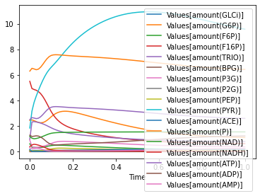
so lets plot just the amounts we got:
[9]:
amount_columns = list(df.columns)
amount_columns = [name for name in amount_columns if 'amount(' in name]
[10]:
df[amount_columns].plot();
of course the added global parameters can be easily removed:
[11]:
remove_amount_expressions()
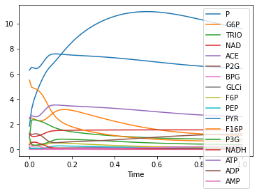
and now we can plot the concentrations:
[14]:
run_time_course(use_sbml_id=True).plot();
[ ]: