Simulating with custom results
In this example, we’ll load a model, and simulate it, fine tuning the simulation results returned. We start as usual:
[1]:
from basico import *
lets load a model, i’ll choose a model from the BioModels Database:
[2]:
load_biomodel(206);
[3]:
get_species()
[3]:
| compartment | type | unit | initial_concentration | initial_particle_number | initial_expression | expression | concentration | particle_number | rate | particle_number_rate | key | sbml_id | |
|---|---|---|---|---|---|---|---|---|---|---|---|---|---|
| name | |||||||||||||
| ATP | compartment | reactions | mmol/l | 2.00 | 1.204428e+21 | NaN | NaN | 0.0 | 0.0 | Metabolite_1 | at | ||
| Triose_Gly3Phos_DHAP | compartment | reactions | mmol/l | 0.60 | 3.613284e+20 | NaN | NaN | 0.0 | 0.0 | Metabolite_3 | s3 | ||
| Acetaldehyde | compartment | reactions | mmol/l | 0.08 | 4.817713e+19 | NaN | NaN | 0.0 | 0.0 | Metabolite_7 | s6 | ||
| NAD | compartment | reactions | mmol/l | 0.60 | 3.613284e+20 | NaN | NaN | 0.0 | 0.0 | Metabolite_4 | na | ||
| Pyruvate | compartment | reactions | mmol/l | 8.00 | 4.817713e+21 | NaN | NaN | 0.0 | 0.0 | Metabolite_6 | s5 | ||
| Glucose | compartment | reactions | mmol/l | 1.00 | 6.022141e+20 | NaN | NaN | 0.0 | 0.0 | Metabolite_0 | s1 | ||
| extracellular acetaldehyde | compartment | reactions | mmol/l | 0.02 | 1.204428e+19 | NaN | NaN | 0.0 | 0.0 | Metabolite_8 | s6o | ||
| 3PG | compartment | reactions | mmol/l | 0.70 | 4.215499e+20 | NaN | NaN | 0.0 | 0.0 | Metabolite_5 | s4 | ||
| F16P | compartment | reactions | mmol/l | 5.00 | 3.011070e+21 | NaN | NaN | 0.0 | 0.0 | Metabolite_2 | s2 |
[4]:
get_reactions()
[4]:
| scheme | flux | particle_flux | function | key | sbml_id | |
|---|---|---|---|---|---|---|
| name | ||||||
| v1 | Glucose + 2 * ATP = F16P | 0.0 | 0.0 | Function for v1 | Reaction_0 | v1 |
| v2 | F16P = 2 * Triose_Gly3Phos_DHAP | 0.0 | 0.0 | Function for v2 | Reaction_1 | v2 |
| v3 | Triose_Gly3Phos_DHAP + NAD = 3PG + ATP | 0.0 | 0.0 | Function for v3 | Reaction_2 | v3 |
| v4 | 3PG = Pyruvate + ATP | 0.0 | 0.0 | Function for v4 | Reaction_3 | v4 |
| v5 | Pyruvate = Acetaldehyde | 0.0 | 0.0 | Function for v5 | Reaction_4 | v5 |
| v7 | ATP = | 0.0 | 0.0 | Function for v7 | Reaction_5 | v7 |
| v8 | Triose_Gly3Phos_DHAP = NAD | 0.0 | 0.0 | Function for v8 | Reaction_6 | v8 |
| v9 | "extracellular acetaldehyde" = | 0.0 | 0.0 | Function for v9 | Reaction_7 | v9 |
| v10 | Acetaldehyde = 0.1 * "extracellular acetaldehyde" | 0.0 | 0.0 | Function for v10 | Reaction_8 | v10 |
| v6 | Acetaldehyde = NAD | 0.0 | 0.0 | Function for v6 | Reaction_9 | v6 |
| v0 | = Glucose | 0.0 | 0.0 | Constant flux (reversible) | Reaction_10 | v0 |
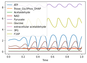
Simulations:
[5]:
run_time_course(duration=1).plot()
[5]:
<AxesSubplot:xlabel='Time'>
Custom Selection list
Sometimes you just want to select certain elements, for which you want to select the output. This can be done using run_time_course_with_output, where the first element is an array of display names, for which you’d like to collect the output
[6]:
run_time_course_with_output(['Time', '[ATP]', 'ATP.Rate', '(v1).Flux'], duration=1)
[6]:
| Time | [ATP] | ATP.Rate | (v1).Flux | |
|---|---|---|---|---|
| 0 | 0.00 | 2.000000 | 23.471501 | 64.705882 |
| 1 | 0.01 | 2.103916 | 23.471501 | 52.477019 |
| 2 | 0.02 | 2.127439 | 23.471501 | 50.238184 |
| 3 | 0.03 | 2.147108 | 23.471501 | 49.133261 |
| 4 | 0.04 | 2.172374 | 23.471501 | 48.222173 |
| ... | ... | ... | ... | ... |
| 96 | 0.96 | 0.700117 | 23.471501 | 58.593102 |
| 97 | 0.97 | 1.226780 | 23.471501 | 40.493568 |
| 98 | 0.98 | 1.833802 | 23.471501 | 29.080133 |
| 99 | 0.99 | 2.349971 | 23.471501 | 24.298749 |
| 100 | 1.00 | 2.708829 | 23.471501 | 23.269926 |
101 rows × 4 columns
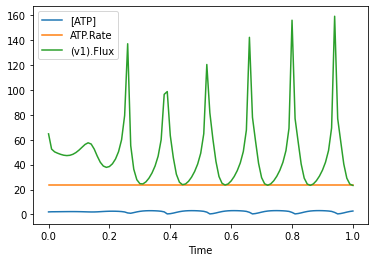
as you see just, as with run_time_course a pandas dataframe is returned, the only difference is, that the index column is not automatically set to the time column (as you might not want to collect time!).
[7]:
run_time_course_with_output(['Time', '[ATP]', 'ATP.Rate', '(v1).Flux'], duration=1).set_index('Time').plot()
[7]:
<AxesSubplot:xlabel='Time'>
The other difference, hen using this method is, that the selection is not automatically saved to COPASI, so when you prepare a model and run it later in the COPASI UI, the output selection is not persisted. You would have to create plot elements or reports for that.
Custom Time Points
Some times you might only want to return values at certain times, this is possible as well (with either run_time_course and run_time_course_with_output, adding the ‘values’ argument:
[8]:
run_time_course(values=[0, 1, 2, 4])
[8]:
| ATP | Triose_Gly3Phos_DHAP | Acetaldehyde | NAD | Pyruvate | Glucose | extracellular acetaldehyde | 3PG | F16P | |
|---|---|---|---|---|---|---|---|---|---|
| Time | |||||||||
| 0.0 | 2.000000 | 0.600000 | 0.080000 | 0.600000 | 8.000000 | 1.000000 | 0.020000 | 0.700000 | 5.000000 |
| 1.0 | 2.708848 | 0.593576 | 0.074087 | 0.579888 | 8.415963 | 0.856600 | 0.023069 | 0.672236 | 5.160410 |
| 2.0 | 3.001586 | 0.574146 | 0.078183 | 0.620547 | 8.217482 | 1.290106 | 0.024351 | 0.848794 | 4.759722 |
| 4.0 | 2.923411 | 0.508574 | 0.080717 | 0.645962 | 8.019722 | 1.851914 | 0.025662 | 0.903727 | 4.376452 |
[9]:
run_time_course_with_output(['Time', '[ATP]', 'ATP.Rate'], values=[0, 1, 2, 4])
[9]:
| Time | [ATP] | ATP.Rate | |
|---|---|---|---|
| 0 | 0.0 | 2.000000 | 23.471501 |
| 1 | 1.0 | 2.708848 | 23.471501 |
| 2 | 2.0 | 3.001586 | 23.471501 |
| 3 | 4.0 | 2.923411 | 23.471501 |
For expert users
For some elements, we do not have an easy mapping between object and display names, to help around that issue run_time_course_with_output allows the use of CN’s as well. Though of course they are quite error prone and not as nice to read!
[10]:
run_time_course_with_output([
    'CN=Root,Model=Wolf2000_Glycolytic_Oscillations,Reference=Time',
    'CN=Root,Model=Wolf2000_Glycolytic_Oscillations,Vector=Compartments[compartment],Vector=Metabolites[Glucose],Reference=ParticleNumber',
    'CN=Root,Model=Wolf2000_Glycolytic_Oscillations,Vector=Compartments[compartment],Reference=Volume'],
    values=[0, 1, 2, 4])
[10]:
| Time | Glucose.ParticleNumber | Compartments[compartment].Volume | |
|---|---|---|---|
| 0 | 0.0 | 6.022141e+20 | 1.0 |
| 1 | 1.0 | 5.158565e+20 | 1.0 |
| 2 | 2.0 | 7.769203e+20 | 1.0 |
| 3 | 4.0 | 1.115249e+21 | 1.0 |
[ ]: