Simple simulations and plotting
In this file, we load a model from the BioModels database, and simulate it for varying durations. We start as usual:
[2]:
from basico import *
Load a model
to load the model, we use the load_biomodel function, it takes in either an integer, which will be transformed into a valid biomodels id, or you can pass in a valid biomodels id to begin with:
[3]:
biomod = load_biomodel(10)
Run time course
After the model is loaded, it is ready to be simulated, here we try it for varying durations:
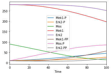
Time course duration 100
[4]:
tc = run_time_course(duration = 100)
tc.plot();
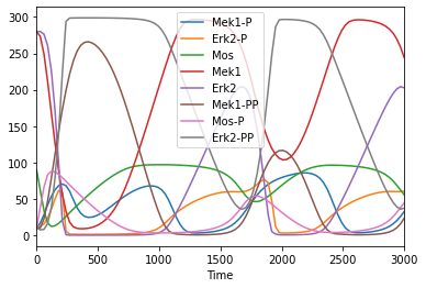
Time course duration 3000
[5]:
tc = run_time_course(duration = 3000)
tc.plot();
Get compartments
To get an overview of what elements the model entails, we can query the individual elements, yielding each time a pandas dataframe with the information:
[6]:
get_compartments()
[6]:
| type | unit | initial_size | initial_expression | dimensionality | expression | size | rate | key | |
|---|---|---|---|---|---|---|---|---|---|
| name | |||||||||
| uVol | fixed | l | 1.0 | 3 | 1.0 | 0.0 | Compartment_0 |
Get parameters (“global quantities”)
[7]:
get_parameters() # no global quantities
Run steady state
we can also run the model to steady state, in order to see the steady state concentrations:
[9]:
run_steadystate()
# now call get_species, to get the steady state concentration and particle numbers
get_species()[['concentration', 'particle_number']]
[9]:
| compartment | type | unit | initial_concentration | initial_particle_number | initial_expression | expression | concentration | particle_number | rate | particle_number_rate | key | |
|---|---|---|---|---|---|---|---|---|---|---|---|---|
| name | ||||||||||||
| Mek1-P | uVol | reactions | nmol/l | 10.0 | 6.022141e+15 | 41.142140 | 2.477638e+16 | 3.113511e-16 | 0.187500 | Metabolite_3 | ||
| Erk2-P | uVol | reactions | nmol/l | 10.0 | 6.022141e+15 | 99.971352 | 6.020416e+16 | 0.000000e+00 | 0.000000 | Metabolite_6 | ||
| Mos | uVol | reactions | nmol/l | 90.0 | 5.419927e+16 | 76.635083 | 4.615073e+16 | -7.783777e-17 | -0.046875 | Metabolite_0 | ||
| Mek1 | uVol | reactions | nmol/l | 280.0 | 1.686199e+17 | 238.913726 | 1.438772e+17 | 0.000000e+00 | 0.000000 | Metabolite_2 | ||
| Erk2 | uVol | reactions | nmol/l | 280.0 | 1.686199e+17 | 102.158541 | 6.152131e+16 | -6.745940e-16 | -0.406250 | Metabolite_5 | ||
| Mek1-PP | uVol | reactions | nmol/l | 10.0 | 6.022141e+15 | 19.944135 | 1.201064e+16 | -3.113511e-16 | -0.187500 | Metabolite_4 | ||
| Mos-P | uVol | reactions | nmol/l | 10.0 | 6.022141e+15 | 23.364917 | 1.407068e+16 | 7.783777e-17 | 0.046875 | Metabolite_1 | ||
| Erk2-PP | uVol | reactions | nmol/l | 10.0 | 6.022141e+15 | 97.870107 | 5.893876e+16 | 6.745940e-16 | 0.406250 | Metabolite_7 |
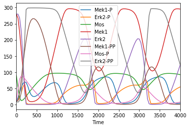
Use pandas syntax for indexing and plotting
[10]:
tc = run_time_course(model = biomod, duration = 4000)
tc.plot();
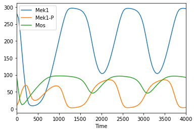
[11]:
tc.loc[:, ['Mek1', 'Mek1-P', 'Mos']].plot()
[11]:
<AxesSubplot:xlabel='Time'>