Creating and simulating a simple model
Here we show how to create a basic model using basiCO, and simulating it. We start as usual by importing basiCO.
[1]:
import sys
if '../..' not in sys.path:
    sys.path.append('../..')
try:
  from basico import *
except ImportError:
  !pip install -q copasi-basico
  from basico import *
import numpy as np
import matplotlib.pyplot as plt
%matplotlib inline
Now lets create a new model, passing along the name that we want to give it. Additional supported parameters for the model consist of:
quantity_unit: which sets the unit to use for species concentrations (defaults to mol)volume_unit: the unit to use for three dimensional compartments (defaults to litre (l))time_unit: the unit to use for time (defaults to second (s))area_unit: the unit to use for two dimensional compartmentslength_unit: the unit to use for one dimensional compartments
[2]:
new_model(name='Simple Model');
now we add a basic reaction that converts a chemical species A irreversibly into B. We can do that by just calling addReaction with the chemical formula to use. In this case this would be: A -> B. The reaction will be automatically created using mass action kinetics.
[3]:
add_reaction('R1', 'A -> B');
Since we had a new model, this created the Species A and B as well as a compartment compartment, in which those chemicals reside. The species have an initial concentration of 1. To verify we can call get_species, which returns a dataframe with all information about the species (either all species, or the one filtered to):
[4]:
get_species().initial_concentration
[4]:
name
A    1.0
B    1.0
Name: initial_concentration, dtype: float64
to change the initial concentration, we use set_species, and specify which property we want to change:
[5]:
set_species('B', initial_concentration=0)
set_species('A', initial_concentration=10)
get_species().initial_concentration
[5]:
name
A    10.0
B     0.0
Name: initial_concentration, dtype: float64
to see the kinetic paramters of our recation we can use get_reaction_parameters, and we see that the parameter has been created by default with a value of 0.1
[6]:
get_reaction_parameters()
[6]:
| value | reaction | type | mapped_to | |
|---|---|---|---|---|
| name | ||||
| (R1).k1 | 0.1 | R1 | local |
to change that parameter, we use set_reaction_parameters, specifying the value to be changed:
[7]:
set_reaction_parameters('(R1).k1', value=1)
get_reaction_parameters('k1')
[7]:
| value | reaction | type | mapped_to | |
|---|---|---|---|---|
| name | ||||
| (R1).k1 | 1.0 | R1 | local |
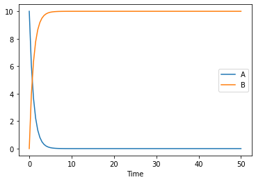
now lets simulate our model for 10 seconds:
[8]:
result = run_time_course(duration=50)
result.plot();
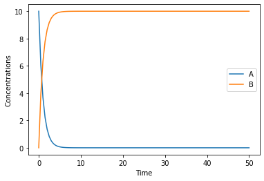
this basic plot is done by pandas, and returns a matplotlib.axes.AxesSubplot object, that can be used to modify it further (full documantation is in the pandas documentation), if you wanted to change the Y label for example you could run:
[9]:
ax = result.plot();
ax.set_ylabel('Concentrations');
to simulate the model stochastically, you can specify the simulation method. COPASI supports many different simulations methods:
deterministic: using the COPASI LSODA implementationstochastic: using the Gibson Bruck algorithmdirectMethod: using the Gillespie direct method
others are:
tauleap,adaptivesa,radau5,hybridlsoda,hybridode45
So lets try and simulate the model stochastically:
[10]:
result = run_time_course(duration=50, method='stochastic')
Error while initializing the simulation: >ERROR 2023-08-10T13:20:07<
  At least one particle number in the initial state is too big.
simulation failed in this time because the particle numbers, that the stochastic simulation is based upon is too high! Lets check:
[11]:
get_species().initial_particle_number
[11]:
name
A    6.022141e+24
B    0.000000e+00
Name: initial_particle_number, dtype: float64
so we just set the initial particle number of a to be smaller, and run the simulation again, this time returning particle numbers rather than concentrations for the resulting dataframe
[12]:
set_species('A', initial_particle_number=100)
Alternatively we could have modified the models quantity unit, which currently was set to:
[13]:
get_model_units()
[13]:
{'time_unit': 's',
 'quantity_unit': 'mol',
 'length_unit': 'm',
 'area_unit': 'm²',
 'volume_unit': 'l'}
So initially we had a concentration of 10 mol/l, which does not lend itself for stochastic simulation. Using the set_model_unit command with a more apropriate quantity_unit and volume_unit would be the propper solution.
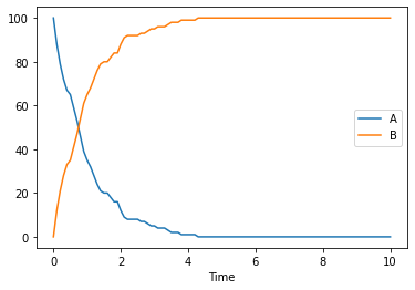
When running stochastic simulations, you might want to specify the seed to be used, so that traces become reproducible. In COPASI you have two parameters for that seed, the actual seed, and use_seed a boolean indicating whether that seed is to be used for the next simulation. For a single trace we use both:
[14]:
result = run_time_course(duration=10, method='stochastic', use_numbers=True, seed=1234, use_seed=True)
result.plot();
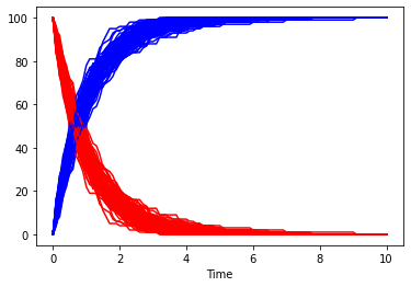
of course one stochastic trace will not be enough, so lets run many of them. This time the species will be plotted separately, so that it is easy to reuse the same color. This time we also don’t use the seed specified before.
[15]:
fig, ax = plt.subplots()
for i in range(100):
    result = run_time_course(duration=10, method='stochastic', use_numbers=True, use_seed=False)
    result.plot(y='A', color='r', ax=ax, legend=None);
    result.plot(y='B', color='b', ax=ax, legend=None);
so far, we were only using mass action kinetics, but of course we could use any other kinetic as well. COPASI comes with a large number of functions already inbuilt. You can see those, running the get_functions command. It is filterable by name, and whether or not the formula is reversible, or general (general reactions can be used for either reversibility). Since we modelled our reaction as irreversible, lets look at the irreversible functions we have:
[16]:
get_functions(reversible=False)
[16]:
| reversible | formula | general | mapping | |
|---|---|---|---|---|
| name | ||||
| Allosteric inhibition (MWC) | False | V*(substrate/Ks)*(1+(substrate/Ks))^(n-1)/(L*(... | False | {'substrate': 'substrate', 'Inhibitor': 'modif... |
| Catalytic activation (irrev) | False | V*substrate*Activator/((Kms+substrate)*(Ka+Act... | False | {'substrate': 'substrate', 'Activator': 'modif... |
| Competitive inhibition (irr) | False | V*substrate/(Km+substrate+Km*Inhibitor/Ki) | False | {'substrate': 'substrate', 'Inhibitor': 'modif... |
| Constant flux (irreversible) | False | v | False | {'v': 'parameter'} |
| Henri-Michaelis-Menten (irreversible) | False | V*substrate/(Km+substrate) | False | {'substrate': 'substrate', 'Km': 'parameter', ... |
| Hill Cooperativity | False | V*(substrate/Shalve)^h/(1+(substrate/Shalve)^h) | False | {'substrate': 'substrate', 'Shalve': 'paramete... |
| Hyperbolic modifier (irrev) | False | V*substrate*(1+b*Modifier/(a*Kd))/(Km*(1+Modif... | False | {'substrate': 'substrate', 'Modifier': 'modifi... |
| Mass action (irreversible) | False | k1*PRODUCT<substrate_i> | False | {'k1': 'parameter', 'substrate': 'substrate'} |
| Mixed activation (irrev) | False | V*substrate*Activator/(Kms*(Kas+Activator)+sub... | False | {'substrate': 'substrate', 'Activator': 'modif... |
| Mixed inhibition (irr) | False | V*substrate/(Km*(1+Inhibitor/Kis)+substrate*(1... | False | {'substrate': 'substrate', 'Inhibitor': 'modif... |
| Noncompetitive inhibition (irr) | False | V*substrate/((Km+substrate)*(1+Inhibitor/Ki)) | False | {'substrate': 'substrate', 'Inhibitor': 'modif... |
| Specific activation (irrev) | False | V*substrate*Activator/(Kms*Ka+(Kms+substrate)*... | False | {'substrate': 'substrate', 'Activator': 'modif... |
| Substrate activation (irr) | False | V*(substrate/Ksa)^2/(1+substrate/Ksc+substrate... | False | {'substrate': 'substrate', 'V': 'parameter', '... |
| Substrate inhibition (irr) | False | V*substrate/(Km+substrate+Km*(substrate/Ki)^2) | False | {'substrate': 'substrate', 'Km': 'parameter', ... |
| Uncompetitive inhibition (irr) | False | V*substrate/(Km+substrate*(1+Inhibitor/Ki)) | False | {'substrate': 'substrate', 'Inhibitor': 'modif... |
| Bi (irreversible) | False | vmax*A*B/(Kma*Kmb + A*Kmb + B*Kma + A*B) | False | {'vmax': 'parameter', 'A': 'substrate', 'B': '... |
| Arrhenius Bimolecular (irr) | False | A*exp(-Ea/(R*T))*S1*S2 | False | {'A': 'parameter', 'Ea': 'parameter', 'R': 'pa... |
| Arrhenius Unimolecular (irr) | False | A*exp(-Ea/(R*T))*S | False | {'A': 'parameter', 'Ea': 'parameter', 'R': 'pa... |
So lets change the kinetic function that our reaction should use. Here we simply specify the function name that we got from the call before. This will introduce new local parameters, for Km and Vmax to the model. (We of course could have used the function parameter already add the add_reaction command above.
[17]:
set_reaction('R1', function='Henri-Michaelis-Menten (irreversible)')
[18]:
get_reactions()
[18]:
| scheme | flux | particle_flux | function | key | sbml_id | mapping | |
|---|---|---|---|---|---|---|---|
| name | |||||||
| R1 | A -> B | 0.0 | 0.0 | Henri-Michaelis-Menten (irreversible) | Reaction_0 | {'substrate': 'A', 'Km': 0.1, 'V': 0.1} |
[19]:
get_reaction_parameters()
[19]:
| value | reaction | type | mapped_to | |
|---|---|---|---|---|
| name | ||||
| (R1).Km | 0.1 | R1 | local | |
| (R1).V | 0.1 | R1 | local |
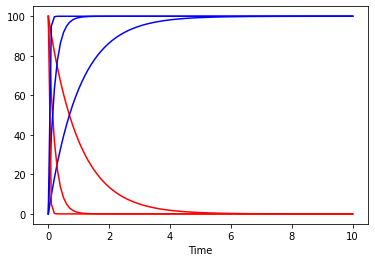
and now we can look at how the plot would look at repeating the simulation for several vmax values:
[20]:
fig, ax = plt.subplots()
for vm in [0.1, 0.5, 3]:
    set_reaction_parameters('(R1).V', value=vm)
    result = run_time_course(duration=10, method='deterministic', use_numbers=True)
    result.plot(y='A', color='r', ax=ax, legend=None);
    result.plot(y='B', color='b', ax=ax, legend=None);